Valuation
A Guide to the DCF
In this article
Overview
The discounted cash flow analysis (DCF analysis) is a way to value companies that uses a foundational idea in corporate finance: things are worth the cash they produce.
The DCF values companies based on the present value of their future cash flows. It buckets the future years of a company’s existence into two groups: (1) a forecast period and (2) everything else. The cash flows from the forecast period years are called the explicitly forecasted free cash flows (or just called “FCF”). The cash flows from remaining years are grouped into one number called the “terminal value”1.
Note that historical cash flows get no credit. We don’t care how much money the company made in the past, only how much it will make in the future. Historical financials are mainly useful to inform our projections.
Discount Rates
After projecting FCF and calculating terminal value, we have to discount all of it to the present value. Discounting is necessary because money today is more valuable than the same amount of money tomorrow. This is due to opportunity cost (common wrong answer is “inflation”). You can take $100, put it in US treasury bills, and make about 4% on it each year with basically no risk. The opportunity cost, though, isn’t the same if you add risk. If there’s a chance you might lose money, then just to break even, you need to get paid more than the 4% the government will give you.
This is why future cash is not taken at face value: (1) present cash can generate returns and (2) those returns are proportional to the risk you take. Future cash must be adjusted for opportunity cost.
Discounting is the act of adjusting future cash flows for opportunity cost (and therefore risk). In the DCF, we calculate a discount rate and then discount future cash flows to make sure our results take into account the risk of that investment.
There are two ways to set up a DCF:
- Project unlevered free cash flow (UFCF); use the weighted average cost of capital (WACC) as the discount rate. The output of the DCF is enterprise value.
- Project levered free cash flow (LFCF); use the cost of equity (CoE or ) as the discount rate. The output of the DCF is equity value.
This pairing is intentional and should not be shuffled. UFCF includes cash flow that belongs to all capital providers (shareholders and creditors) because to calculate it, you don’t subtract out interest expense. WACC is the discount rate that includes the cost of all sources of capital. LFCF only includes cash flow that belongs to shareholders (its calculation includes the subtraction of interest expense). CoE is the discount rate that only considers the cost of capital from shareholders.
The actual way you discount future cash flows is by calculating the discount factor:
This comes out of the present-value formula, which is itself just a rearrangement of the easier-to-understand relationship that a present amount, grown at the discount rate, equals its future value:
Once you have the explicit FCF forecast and the discount factor, you simply multiply them and sum them up to get the NPV of FCF.
Calculating Free Cash Flow
Both UFCF and LFCF start the same way. You begin with revenue and then subtract the cost of goods sold and operating expenses: this results in operating income (i.e., EBIT). From there, to get to UFCF, you multiply it by (1 − Tax Rate) to get a tax-impacted figure called net operating profit after tax (NOPAT). From NOPAT, you add D&A, subtract capital expenditures, and subtract the change in net working capital2:
To get from EBIT to LFCF the process is the same, except you first subtract interest expense before taking out taxes:
That is the simplified version, and it is the one most interviewers want. Some will push for mandatory debt repayments to come out as well, with any new debt raised added back, on the reasoning that principal owed to lenders was never available to shareholders in the first place. If you are asked for the full build, subtract mandatory amortization and add new borrowing.
Terminal Value
There are two ways to calculate terminal value: the perpetuity growth method (also called the Gordon growth method) and the exit multiple method. The perpetuity growth method assumes:
- The company exists forever.
- Its FCF grows forever at a certain rate called the perpetuity growth rate (PGR).
- That FCF continues to be discounted forever at the discount rate.
When you use the perpetuity growth method, the terminal value is a geometric series (a sum where the pattern is ). Because the discount rate is higher than the perpetuity growth rate, the series eventually converges (i.e., terms get smaller and smaller until it basically hits zero, which means the sum is not infinity). The formula for terminal value using the perpetuity growth rate is:
What is a reasonable value for the perpetuity growth rate? It cannot be greater than long-term nominal GDP growth (~4% is the latest FOMC estimate, with 2% inflation and 2% real GDP growth) because if a company grows every year for eternity faster than the economy, at some point the company will exceed the size of the economy. People commonly use 2–3%, with the typical explanation being that it reflects real GDP growth or inflation. A key note is that not all businesses get the same PGR. This is an input that requires judgment like everything else in the DCF. A business that is very unlikely to grow after the explicit forecast period should get close to a 0% PGR. A fast grower could get something closer to nominal GDP for its PGR.
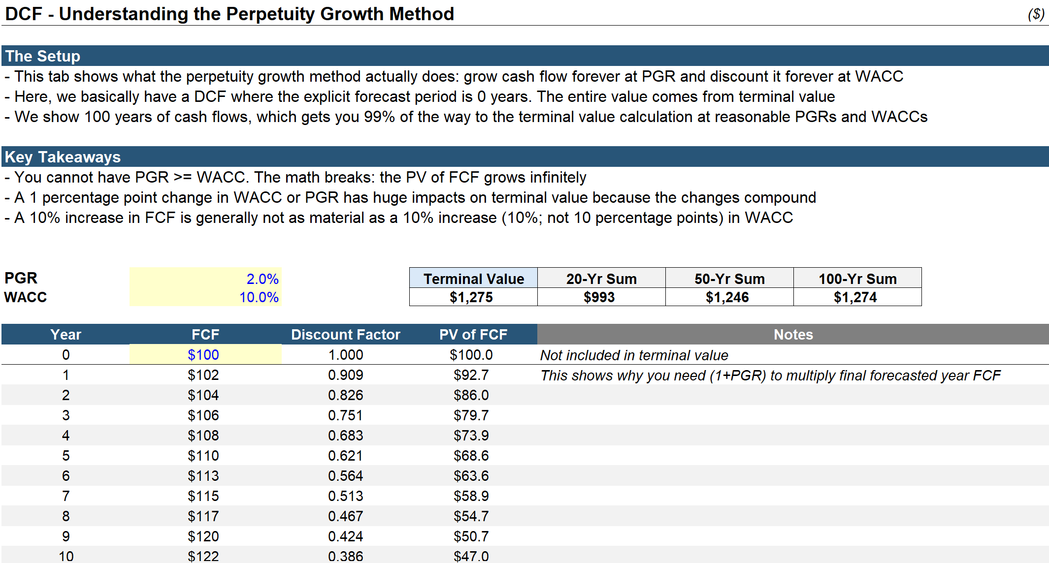
The DCF Excel includes a tab to help understand the perpetuity growth method better.
The exit multiple method is much simpler than the perpetuity growth method. You get valuation multiples from precedent transactions or comparable companies and apply them to the final projected year’s figures. So if 5 peers were acquired at a median of 10x LTM EBITDA, we apply 10x to the final projected year’s EBITDA. There are some nuances, though. First, the peers chosen should ideally have a similar maturity as the target company at the end of the explicit forecast period, not its maturity today. Second, the use of precedent transactions instead of comparable companies might not be appropriate depending on the context of our analysis: precedent transaction multiples will include control premiums. Third, exit multiples need to be sanity checked by calculating the implied PGR from an exit multiple. The intuition behind the math is easy: you have two formulas that equal each other. Just solve for PGR.
Show the full derivation: implied PGR from an exit multiple (7 steps)
You don’t need to memorize this. Set the two terminal-value formulas equal and solve for PGR.
- 1
- 2
- 3
- 4
- 5
- 6
- 7
You don’t need to know this formula connecting the two methods but you should know each individual terminal value formula and the idea behind how to link them.
Regardless of how the terminal value is calculated, it needs to be discounted. The perpetuity growth method calculates terminal value from the end of the explicit forecast period. The exit multiple method assumes that the company is sold at the end of the explicit forecast period. They are both lumps of cash as of the end of the explicit forecast period. So we use the discount factor corresponding to that.
WACC
The WACC is well-named. The formula is intuitive: multiply how much each part of the capital structure costs by what percentage of the capital structure it is.
If the capital structure includes preferred equity, you just add the cost of preferred and the percentage of capital from preferred as well. The (1 − Tax Rate) attached to debt is because the cost of debt reflects the interest expense, which is tax-deductible. So the effective cost of debt is lower than it first appears.
The cost of equity is not as straightforward as debt, both to understand and to calculate. Here we have to return to the opportunity cost idea: for an equity investor to give a company capital, they must expect that they will at least get compensated for the risk they’re taking.
The cost of equity formula assumes the risk of each company is just some multiple of the overall stock market’s risk. Beta is that multiple. The overall risk of the stock market is the equity risk premium, which is simply the return of the stock market over the risk-free rate.
Result of a DCF
The immediate output of a DCF depends on whether it was built with UFCF or LFCF. With UFCF, it outputs enterprise value; with LFCF, it outputs equity value. The enterprise value DCF can be (and often is) used to calculate equity value simply by bridging from EV to EqV. A big advantage of the UFCF DCF is that you don’t have to project interest expenses, which can take longer to build and typically introduces circularity into the model3.
Midyear Convention
Midyear convention is an important adjustment used in most real DCFs. For most companies, cash flow is generated somewhat evenly across the year. But when you have whole-number discounting periods, you end up discounting each year’s cash flows as if they all land at the end of the year: this leads to over-discounting and therefore underestimating company value. Therefore you make an adjustment: for every period, you discount as if the cash flows all land halfway through the period. So instead of Year 1 getting discounted as period 1, it’s discounted as period 0.5.
The midyear convention applies differently to the terminal value depending on what method is used. If using the perpetuity growth rate, you just discount it at the same discount factor as the final explicitly projected year. But if using the exit multiple method, you discount it as if the terminal value comes from the end of the period: not the half-year. So if the final explicitly projected year’s discount period is 4.5, the terminal value (exit mult. method) is discounted at period 5. The reason is that the financials (the EBIT or EBITDA figure) used to calculate terminal value are full-year if using the exit multiple method.
Forecast Length
The standard wisdom is that a DCF should have an explicit forecast of 5 to 10 years. If you forecast fewer than 5 years, the explicit forecast is so short that the NPV of FCF will likely be too small relative to the terminal value: at that point you might as well not do a DCF and instead take a multiples-based approach. A forecast greater than 10 years is too difficult (even forecasting 10 years out with much confidence is hard). At some point you have to admit that you lack insight into the granular cost structure details of a company X years from now. That is why both terminal value methods are so fundamentally simple and require so few inputs: they reflect a lack of information.
Relatedly, a DCF is likely over-reliant on terminal value if over 80% of enterprise value comes from terminal value.
Next Steps
The nuances of a DCF and all financial models are best understood in Excel, not with books or articles. The right approach is to (1) understand the concepts, (2) look at an actual DCF, (3) recreate it, and (4) check your work. A DCF can be hundreds of rows or 10 rows. Our reference DCF has multiple versions, ranging from a lightweight toy you can understand in 5 minutes to something closer to a real DCF.
Learning the DCF (Excel workbook)Levels 0–3, from a 10-row toy to a near-real DCF · .xlsxDownloadFootnotes
- This nomenclature is shorthand that by itself isn’t entirely conceptually accurate. Terminal value also reflects the value of free cash flow, just with simplifications. The first category should really be called “explicitly projected FCF” but that’s too much of a mouthful so we short-hand it. ↩
- In valuation, we always use operating net working capital, not the accounting definition. Net working capital is current assets − current liabilities. But “current assets” includes cash. “current liabilities” includes short-term debt. For valuation, that’s not good. We need to strip out cash and debt/debt-like items. The accounting version of NWC shows you liquidity. Operating NWC shows you the short-term sources and uses of cash in the day-to-day business buying and selling stuff. In banking, always assume that when someone says NWC they mean operating NWC unless they explicitly state otherwise. ↩
- The UFCF DCF requires the EV-EqV bridge and the non-equity components of WACC, but the EV-EqV bridge is quick (usually you have to build it somewhere else anyway during analysis) and CoE is the hardest part of the WACC calculation anyway, and the rest of WACC is usually easy. ↩